- Power BI forums
- Updates
- News & Announcements
- Get Help with Power BI
- Desktop
- Service
- Report Server
- Power Query
- Mobile Apps
- Developer
- DAX Commands and Tips
- Custom Visuals Development Discussion
- Health and Life Sciences
- Power BI Spanish forums
- Translated Spanish Desktop
- Power Platform Integration - Better Together!
- Power Platform Integrations (Read-only)
- Power Platform and Dynamics 365 Integrations (Read-only)
- Training and Consulting
- Instructor Led Training
- Dashboard in a Day for Women, by Women
- Galleries
- Community Connections & How-To Videos
- COVID-19 Data Stories Gallery
- Themes Gallery
- Data Stories Gallery
- R Script Showcase
- Webinars and Video Gallery
- Quick Measures Gallery
- 2021 MSBizAppsSummit Gallery
- 2020 MSBizAppsSummit Gallery
- 2019 MSBizAppsSummit Gallery
- Events
- Ideas
- Custom Visuals Ideas
- Issues
- Issues
- Events
- Upcoming Events
- Community Blog
- Power BI Community Blog
- Custom Visuals Community Blog
- Community Support
- Community Accounts & Registration
- Using the Community
- Community Feedback
Register now to learn Fabric in free live sessions led by the best Microsoft experts. From Apr 16 to May 9, in English and Spanish.
- Power BI forums
- Forums
- Get Help with Power BI
- Desktop
- Month columns in excel to create common axis bar c...
- Subscribe to RSS Feed
- Mark Topic as New
- Mark Topic as Read
- Float this Topic for Current User
- Bookmark
- Subscribe
- Printer Friendly Page
- Mark as New
- Bookmark
- Subscribe
- Mute
- Subscribe to RSS Feed
- Permalink
- Report Inappropriate Content
Month columns in excel to create common axis bar chart
I have data set in excel which has month as columns, and merged cells on top of months classify those into Target/ Actuals/ Estimate
Target Actuals Estimates
Project Jan Feb Mar Apr Jan Feb Mar Apr May June July
A
B
My question - I want to create a bar chart with months as common axis and with cumulative values and actual values as Y axis (attached screenshot), Somehow do I need to unpivote data, how can I ? I also need to calculate the cumulative vanues by month using DAX (I have formula but need to understand how can I use it as currently months are columns)
Solved! Go to Solution.
- Mark as New
- Bookmark
- Subscribe
- Mute
- Subscribe to RSS Feed
- Permalink
- Report Inappropriate Content
Hello @HP20 ,
When importing data into Power Query, ensure that there is no merging of your headers
If it is a table, then it should look something like this:
Please apply the following steps in the Power Query:
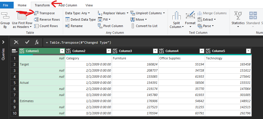
- Transform > Transpose
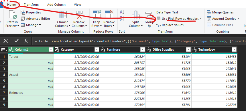
- Home > Use the First Row as Headers
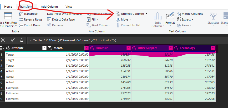
- Select the first column and Fill down:
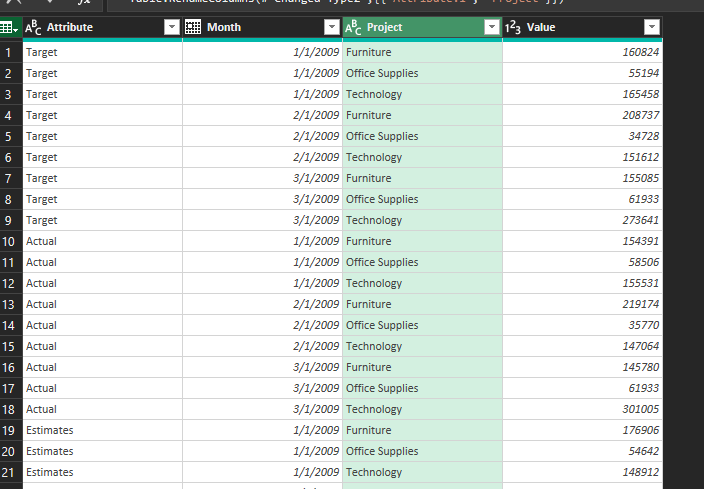
- Select the three columns for project and unpivot
Output:
Hope this helps!
Cheers!
Vivek
Blog: vivran.in/my-blog
Connect on LinkedIn
Follow on Twitter
- Mark as New
- Bookmark
- Subscribe
- Mute
- Subscribe to RSS Feed
- Permalink
- Report Inappropriate Content
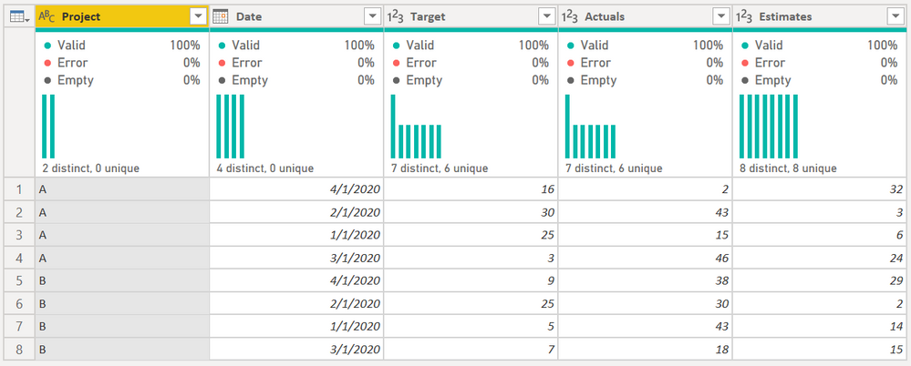
Hi @HP20 - You can try this. This will work even if your headers in Excel are merged. It will transform this:
into this:
The full M code is this:
let
    Source = Excel.Workbook(File.Contents("C:\Users\Ed Hansberry\OneDrive\Work Stuff\Power BI Forum Examples\Test Files\Pivot Data.xlsx"), null, true),
    Sheet1_Sheet = Source{[Item="Sheet1",Kind="Sheet"]}[Data],
    #"Transposed Table" = Table.Transpose(Sheet1_Sheet),
    #"Filled Down" = Table.FillDown(#"Transposed Table",{"Column1"}),
    #"Merged Columns" = Table.CombineColumns(#"Filled Down",{"Column1", "Column2"},Combiner.CombineTextByDelimiter(":", QuoteStyle.None),"Merged"),
    #"Transposed Table1" = Table.Transpose(#"Merged Columns"),
    #"Promoted Headers" = Table.PromoteHeaders(#"Transposed Table1", [PromoteAllScalars=true]),
    #"Unpivoted Other Columns" = Table.UnpivotOtherColumns(#"Promoted Headers", {":Project"}, "Attribute", "Value"),
    #"Split Column by Delimiter" = Table.SplitColumn(#"Unpivoted Other Columns", "Attribute", Splitter.SplitTextByDelimiter(":", QuoteStyle.Csv), {"Attribute.1", "Attribute.2"}),
    #"Pivoted Column" = Table.Pivot(#"Split Column by Delimiter", List.Distinct(#"Split Column by Delimiter"[Attribute.1]), "Attribute.1", "Value"),
    #"Added Custom" = Table.AddColumn(#"Pivoted Column", "Date", each Date.FromText([Attribute.2] & "1, 2020"), type date
),
    #"Renamed Columns" = Table.RenameColumns(#"Added Custom",{{":Project", "Project"}}),
    #"Changed Type" = Table.TransformColumnTypes(#"Renamed Columns",{{"Target", Int64.Type}, {"Actuals", Int64.Type}, {"Estimates", Int64.Type}, {"Project", type text}}),
    #"Removed Other Columns" = Table.SelectColumns(#"Changed Type",{"Project", "Date", "Target", "Actuals", "Estimates"})
in
    #"Removed Other Columns"
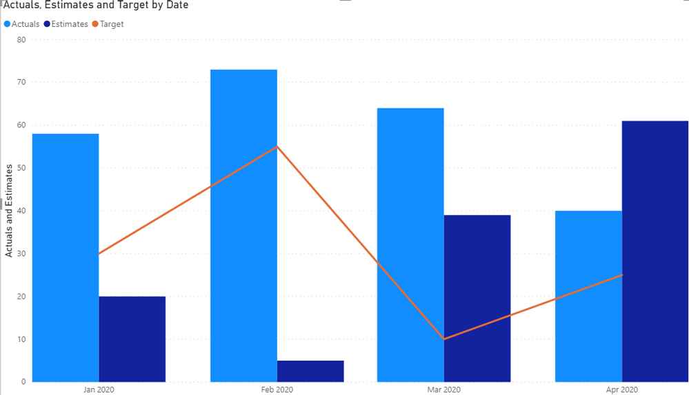
If you copy and paste that into your Blank Query (directions below) and use this Excel file as your source you will be able to walk through the steps as to how I got there. You can then get a visual that looks like this:
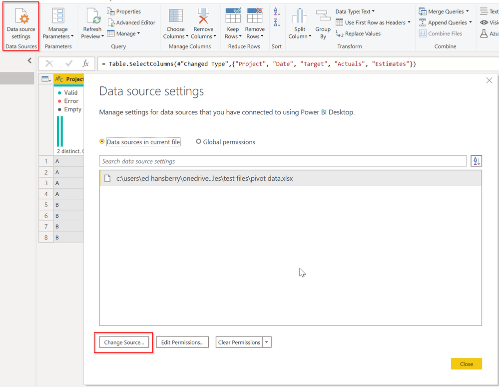
My PBIX file is here. Once you have both the PBIX file and Excel file (linked above) you can change the source for the file to point to the Excel file on your hard drive, then Power Query will work.
If you need further help, please post some good sample data using the links below, not just text in the text box. You'll note I arbitrarly set the date to be the first of the month for 2020. If you have more data we may be able to create a better date that is more intelligent and will adapt to future years.
How to get good help fast. Help us help you.
How to Get Your Question Answered Quickly
How to provide sample data in the Power BI Forum
How to use M code provided in a blank query:
1) In Power Query, select New Source, then Blank Query
2) On the Home ribbon, select "Advanced Editor" button
3) Remove everything you see, then paste the M code I've given you in that box.
4) Press Done
5) See this article if you need help using this M code in your model.
One final note, you can see in my quick model I did not include a date table. you should have one really, and this link will help you create one in Power Query. Then you would use the date from the date table in your visual, and hide the date column in your FACT table. Creating a Dynamic Date Table in Power Query
Did I answer your question? Mark my post as a solution!
Did my answers help arrive at a solution? Give it a kudos by clicking the Thumbs Up!
DAX is for Analysis. Power Query is for Data Modeling
Proud to be a Super User!
MCSA: BI Reporting- Mark as New
- Bookmark
- Subscribe
- Mute
- Subscribe to RSS Feed
- Permalink
- Report Inappropriate Content
Hi,
My Blog article here should help you - Rearrange a multi heading dataset into a single heading one which is Pivot ready.
Regards,
Ashish Mathur
http://www.ashishmathur.com
https://www.linkedin.com/in/excelenthusiasts/
- Mark as New
- Bookmark
- Subscribe
- Mute
- Subscribe to RSS Feed
- Permalink
- Report Inappropriate Content
Hi @HP20 - You can try this. This will work even if your headers in Excel are merged. It will transform this:
into this:
The full M code is this:
let
    Source = Excel.Workbook(File.Contents("C:\Users\Ed Hansberry\OneDrive\Work Stuff\Power BI Forum Examples\Test Files\Pivot Data.xlsx"), null, true),
    Sheet1_Sheet = Source{[Item="Sheet1",Kind="Sheet"]}[Data],
    #"Transposed Table" = Table.Transpose(Sheet1_Sheet),
    #"Filled Down" = Table.FillDown(#"Transposed Table",{"Column1"}),
    #"Merged Columns" = Table.CombineColumns(#"Filled Down",{"Column1", "Column2"},Combiner.CombineTextByDelimiter(":", QuoteStyle.None),"Merged"),
    #"Transposed Table1" = Table.Transpose(#"Merged Columns"),
    #"Promoted Headers" = Table.PromoteHeaders(#"Transposed Table1", [PromoteAllScalars=true]),
    #"Unpivoted Other Columns" = Table.UnpivotOtherColumns(#"Promoted Headers", {":Project"}, "Attribute", "Value"),
    #"Split Column by Delimiter" = Table.SplitColumn(#"Unpivoted Other Columns", "Attribute", Splitter.SplitTextByDelimiter(":", QuoteStyle.Csv), {"Attribute.1", "Attribute.2"}),
    #"Pivoted Column" = Table.Pivot(#"Split Column by Delimiter", List.Distinct(#"Split Column by Delimiter"[Attribute.1]), "Attribute.1", "Value"),
    #"Added Custom" = Table.AddColumn(#"Pivoted Column", "Date", each Date.FromText([Attribute.2] & "1, 2020"), type date
),
    #"Renamed Columns" = Table.RenameColumns(#"Added Custom",{{":Project", "Project"}}),
    #"Changed Type" = Table.TransformColumnTypes(#"Renamed Columns",{{"Target", Int64.Type}, {"Actuals", Int64.Type}, {"Estimates", Int64.Type}, {"Project", type text}}),
    #"Removed Other Columns" = Table.SelectColumns(#"Changed Type",{"Project", "Date", "Target", "Actuals", "Estimates"})
in
    #"Removed Other Columns"
If you copy and paste that into your Blank Query (directions below) and use this Excel file as your source you will be able to walk through the steps as to how I got there. You can then get a visual that looks like this:
My PBIX file is here. Once you have both the PBIX file and Excel file (linked above) you can change the source for the file to point to the Excel file on your hard drive, then Power Query will work.
If you need further help, please post some good sample data using the links below, not just text in the text box. You'll note I arbitrarly set the date to be the first of the month for 2020. If you have more data we may be able to create a better date that is more intelligent and will adapt to future years.
How to get good help fast. Help us help you.
How to Get Your Question Answered Quickly
How to provide sample data in the Power BI Forum
How to use M code provided in a blank query:
1) In Power Query, select New Source, then Blank Query
2) On the Home ribbon, select "Advanced Editor" button
3) Remove everything you see, then paste the M code I've given you in that box.
4) Press Done
5) See this article if you need help using this M code in your model.
One final note, you can see in my quick model I did not include a date table. you should have one really, and this link will help you create one in Power Query. Then you would use the date from the date table in your visual, and hide the date column in your FACT table. Creating a Dynamic Date Table in Power Query
Did I answer your question? Mark my post as a solution!
Did my answers help arrive at a solution? Give it a kudos by clicking the Thumbs Up!
DAX is for Analysis. Power Query is for Data Modeling
Proud to be a Super User!
MCSA: BI Reporting- Mark as New
- Bookmark
- Subscribe
- Mute
- Subscribe to RSS Feed
- Permalink
- Report Inappropriate Content
Thank you I copied my data into your excel file and made few changes in code, it worked perfectly fine..thank you so much @edhans
- Mark as New
- Bookmark
- Subscribe
- Mute
- Subscribe to RSS Feed
- Permalink
- Report Inappropriate Content
Glad I was able to assist @HP20
Did I answer your question? Mark my post as a solution!
Did my answers help arrive at a solution? Give it a kudos by clicking the Thumbs Up!
DAX is for Analysis. Power Query is for Data Modeling
Proud to be a Super User!
MCSA: BI Reporting- Mark as New
- Bookmark
- Subscribe
- Mute
- Subscribe to RSS Feed
- Permalink
- Report Inappropriate Content
Hello @HP20 ,
When importing data into Power Query, ensure that there is no merging of your headers
If it is a table, then it should look something like this:
Please apply the following steps in the Power Query:
- Transform > Transpose
- Home > Use the First Row as Headers
- Select the first column and Fill down:
- Select the three columns for project and unpivot
Output:
Hope this helps!
Cheers!
Vivek
Blog: vivran.in/my-blog
Connect on LinkedIn
Follow on Twitter
- Mark as New
- Bookmark
- Subscribe
- Mute
- Subscribe to RSS Feed
- Permalink
- Report Inappropriate Content
thanks @vivran22 this solution worked too..but as data had merged cells I used the other solution suggested, as I didnt want to add manual step..but this works perfectly fine thanks again!
- Mark as New
- Bookmark
- Subscribe
- Mute
- Subscribe to RSS Feed
- Permalink
- Report Inappropriate Content
- Mark as New
- Bookmark
- Subscribe
- Mute
- Subscribe to RSS Feed
- Permalink
- Report Inappropriate Content
Please confirm if this issue has been resolved. If yes, then mark the appropriate post as a solution as it will help others.
If not, then please share more details along with sample dataset.
Cheers!
Vivek
Blog: vivran.in/my-blog
Connect on LinkedIn
Follow on Twitter
- Mark as New
- Bookmark
- Subscribe
- Mute
- Subscribe to RSS Feed
- Permalink
- Report Inappropriate Content
@HP20 - Short answer is yes, you almost certainly need to unpivot. @ImkeF @edhans might be able to better help with the Power Query to get you there.
@ me in replies or I'll lose your thread!!!
Instead of a Kudo, please vote for this idea
Become an expert!: Enterprise DNA
External Tools: MSHGQM
YouTube Channel!: Microsoft Hates Greg
Latest book!: The Definitive Guide to Power Query (M)
DAX is easy, CALCULATE makes DAX hard...
- Mark as New
- Bookmark
- Subscribe
- Mute
- Subscribe to RSS Feed
- Permalink
- Report Inappropriate Content
Helpful resources

Microsoft Fabric Learn Together
Covering the world! 9:00-10:30 AM Sydney, 4:00-5:30 PM CET (Paris/Berlin), 7:00-8:30 PM Mexico City

Power BI Monthly Update - April 2024
Check out the April 2024 Power BI update to learn about new features.

| User | Count |
|---|---|
| 115 | |
| 100 | |
| 89 | |
| 68 | |
| 61 |
| User | Count |
|---|---|
| 150 | |
| 120 | |
| 100 | |
| 87 | |
| 68 |


