Missed icons for table conditional formatting

[Anonymous]

Hi everybody,

I think my issue is quite simple but I'm really unable to find a solution.

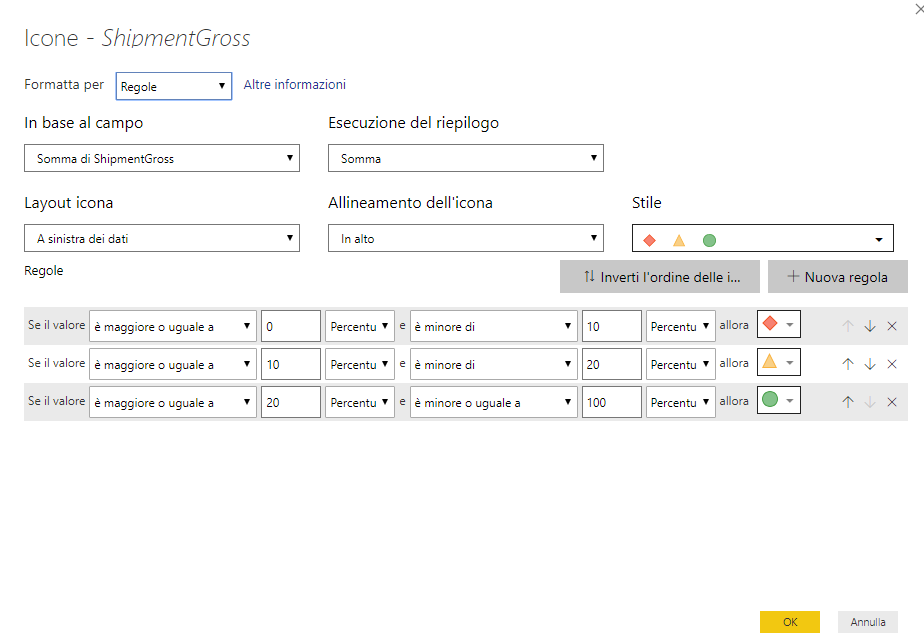
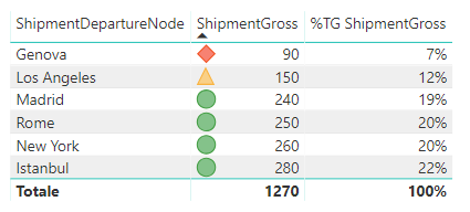
I create a simple table with these data and tried conditional formatting with icons.

So, I don't understand with almost all my icons are green. Values between 127 and 254 would be yellow, but they are not!

What am I missing?

Thank you

[jdbuchanan71]

@Anonymous 

The way the "Percent" conditional formatting works is different than you think, it doesn't have anything to do with percent of total.  It take the lowest and hightest displayed amounts and uses those to determine the formatting bands based on the Percent you entered so your table is looking at these numbers to apply the formatting.

What you want to do is add your value again and display change the "Show value as" > Percent of grand total.

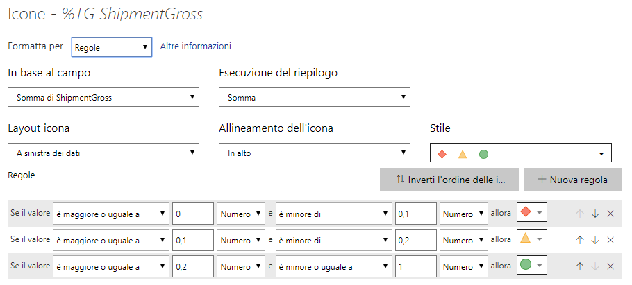
Then apply your conditional formatting to that column based on numbers, not percent.

>= 0, NUMBER  < .1 NUMBER

>= .1 NUMBER  < .2 NUMBER

>= .2 NUMBER  < 1 NUMBER

[Anonymous]

@jdbuchanan71 

It'so weird that percentage conditional formatting works this way. Why would it consider the percentage as the range between maximum and minimum?

Anyway, it explains my icons correctly, but if I try to follow your hint, adding the filed again showing as "Percent of grand total", I don't know how to have conditional formatting based on that percentage:

As you can see, I see no icon while formatting 3rd column of my table. It's because I don't know how to suggest to format based on % of ShipmentGross and not just based on Sum of ShipmentGross.

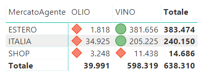
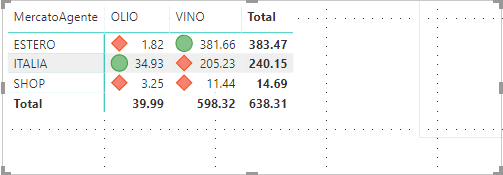
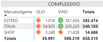
Moreover, if percentual conditional formatting works like you say, why in the following image is 11.438 with red icon? It's the maximum value of its row, so it should be green, and even if it takes max and min from column, than 205.225 should be red.

Thanks you very much for your help

[v-joesh-msft]

Hi @Anonymous ,

The conditional formatting takes the difference between the minimum and maximum values as the cardinality of Percent, not the total.

For the first question, if you want to present the conditional formatting as a percentage of the total, you can try to build a measure, such as the following:

(1)Create a measure to calculate the total percentage：

percentage =
DIVIDE (
    SUM ( test[shipmentgross] ),
    CALCULATE ( SUM ( test[shipmentgross] ), ALLSELECTED( test ) )
)

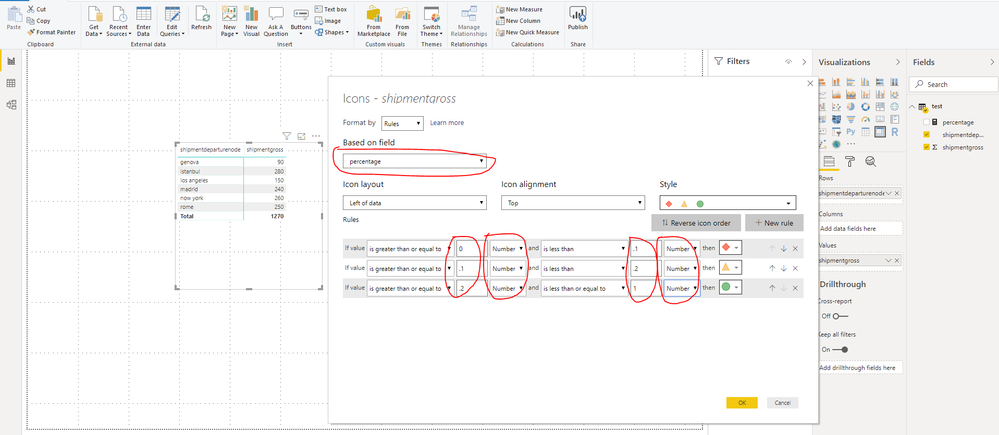
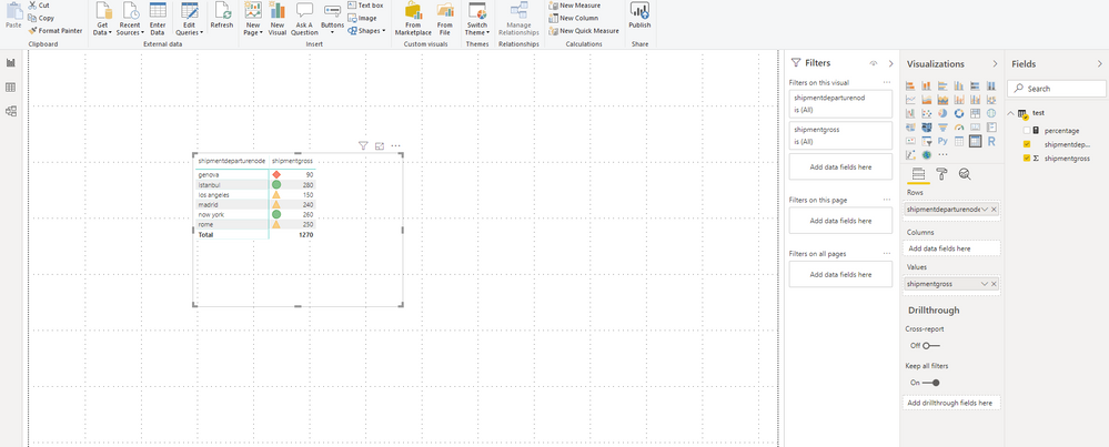
(2) Change the Based on field to “percentage”, change “Percent” to “Number”, and modify the corresponding value. The result is as follows：

For the second question, this involves row context in percent calculation of power bi, please try to use these three measure in conditional formatting:

(1)% CT = DIVIDE(SUM('Table'[Qty]),CALCULATE(SUM('Table'[Qty]),ALLSELECTED('Table'[MercatoAgente])))

(2)% GT = DIVIDE(SUM('Table'[Qty]),CALCULATE(SUM('Table'[Qty]),ALLSELECTED('Table'[Type])))

(3)% RT = DIVIDE(SUM('Table'[Qty]),CALCULATE(SUM('Table'[Qty]),ALLSELECTED('Table')))

Here is demo , please try it：

https://qiuyunus-my.sharepoint.com/:u:/g/personal/pbipro_qiuyunus_onmicrosoft_com/ERTo4bFI8XJJh9v5dmTqo7YB91wWAR_2mHPOvBBMJ4Nqiw?e=GIC8dy

Best Regards,

Community Support Team _ Joey
If this post helps, then please consider Accept it as the solution to help the other members find it more quickly.

[Anonymous]

Thank you @v-joesh-msft 

Now something is brighter to me, but I still have some issue.

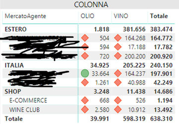
This image shows the table when you use RT measure, it's your 3rd example. Why is 205.225 green? It should be based on percentage based on total (638.310), so it should be red because it's under 50%.

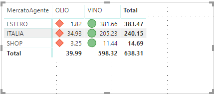
Then, this image shows the table where you used TC (1st example). Why is it all in green? It is based on the column total, so considering SHOP I would expect 668 to be red and 2.580 to be green, related to their column total of 3.248.

Right here, instead, with row total is looks fine, because even with drill down it's green if the value is above 50% of the row total.

Thanks

[v-joesh-msft]

Hi @Anonymous ,

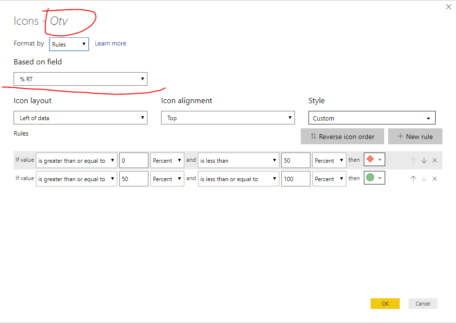
Sorry I made a mistake, you need to set the rules to Number and modify the corresponding value, just like the answer in the first question. The setting of RT/CT/GT is all the same：

Best Regards,

Community Support Team _ Joey
If this post helps, then please consider Accept it as the solution to help the other members find it more quickly.

[Anonymous]

Thank you @v-joesh-msft 

With your hint the example with GT works fine, even if it's weird to see it working while has different conditional formatting settings than RT visual.

Instead, visual with CT is not fine: all the icons stay green! I thought I could need to add Area field (I am drilling down from MercatoAgente to Area) to the ALLSELECTED function in CT measure, but doing it something strange happens:

Some icon colors are good, but why are 2.580 or 200.200 red??

Thanks

[v-joesh-msft]

Hi @ nick93,

I found the formula used in the first answer:：RT with ALLSELECTED('Table')，GT with ALLSELECTED('Table'[Type]) may be confusing, using RT with ALLSELECTED('Table'[Type]), GT with ALLSELECTED('Table') might make a better understanding. RT refers to row total, and GT refers to grand total.

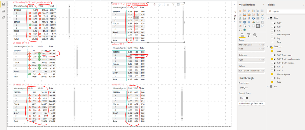
When you add a new field to the row of the matrix, the row context will also change. I have made some examples and hope to have a more intuitive understanding;

1: There is only one field in MercatoAgente in Rows:

2: There are two fields MercatoAgente and Area in Rows:

(1) Presentation of CT/RT/GT:

(2) Presentation of different Rows references in ALLSELECTED:

Looking at the rendering of each of the different fields in the screenshot, you may find the difference and find the result you want.

Here is a demo , please try it：

https://qiuyunus-my.sharepoint.com/:u:/g/personal/pbipro_qiuyunus_onmicrosoft_com/Ea2Xmq1i4N5Kp_U8hS...

Best Regards,

Community Support Team _ Joey
If this post helps, then please consider Accept it as the solution to help the other members find it more quickly.

[Anonymous]

Hi @v-joesh-msft and thank you one more time

Ok, it looks fine, now all what you explained me works.

I have just one last doubt: my aim was to create a conditional formatting which worked fine both if I didn't drill the table down and stayed at MercatoAgente level and if I drilled it down to Area. I would like to create a single measure which formats the table as you see in the following images: in image1 the total to choose the icons should be the column total, in image2 icons should be based on the column total of each MercatoAgente class, and not the whole total.

Image 1: here the ALLSELECTED function contains MercatoAgente

Image 2: here the ALLSELECTED function contains Area

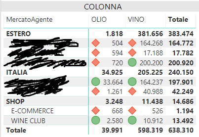
I thought I could create a table formatted this way with a single measure. Is it possible?

Thank you again

[v-joesh-msft · Accepted solution]

Hi @Anonymous ,

You can use the IF statement to nest, and change the measure: "% CT 2 with area" in the previous demo to the following formula：

% CT 2 with area =
IF (
    ISINSCOPE ( 'Table (2)'[ Area] ),
    DIVIDE (
        SUM ( 'Table (2)'[Qty] ),
        CALCULATE ( SUM ( 'Table (2)'[Qty] ), ALLSELECTED ( 'Table (2)'[ Area] ) )
    ),
    DIVIDE (
        SUM ( 'Table (2)'[Qty] ),
        CALCULATE (
            SUM ( 'Table (2)'[Qty] ),
            ALLSELECTED ( 'Table (2)'[MercatoAgente] )
        )
    )
)

Best Regards,

Community Support Team _ Joey
If this post helps, then please consider Accept it as the solution to help the other members find it more quickly.

[Anonymous]

Great @v-joesh-msft, thank you very much!

I would like to mark your answer as the solution but I should log in with my old account (nick93) and right now I have some issues I am trying to solve with Support, so for the moment saldy I can't.

Thanks for your help!

[PattemManohar]

Are you sure that you are conditional formatting is on Percent instead of actual values ? If not, then change the "Percent" to "Number" in the drop-down under Rules.