- Power BI forums
- Updates
- News & Announcements
- Get Help with Power BI
- Desktop
- Service
- Report Server
- Power Query
- Mobile Apps
- Developer
- DAX Commands and Tips
- Custom Visuals Development Discussion
- Health and Life Sciences
- Power BI Spanish forums
- Translated Spanish Desktop
- Power Platform Integration - Better Together!
- Power Platform Integrations (Read-only)
- Power Platform and Dynamics 365 Integrations (Read-only)
- Training and Consulting
- Instructor Led Training
- Dashboard in a Day for Women, by Women
- Galleries
- Community Connections & How-To Videos
- COVID-19 Data Stories Gallery
- Themes Gallery
- Data Stories Gallery
- R Script Showcase
- Webinars and Video Gallery
- Quick Measures Gallery
- 2021 MSBizAppsSummit Gallery
- 2020 MSBizAppsSummit Gallery
- 2019 MSBizAppsSummit Gallery
- Events
- Ideas
- Custom Visuals Ideas
- Issues
- Issues
- Events
- Upcoming Events
- Community Blog
- Power BI Community Blog
- Custom Visuals Community Blog
- Community Support
- Community Accounts & Registration
- Using the Community
- Community Feedback
Register now to learn Fabric in free live sessions led by the best Microsoft experts. From Apr 16 to May 9, in English and Spanish.
- Power BI forums
- Forums
- Get Help with Power BI
- Desktop
- Identify customers who had puchased exactly one un...
- Subscribe to RSS Feed
- Mark Topic as New
- Mark Topic as Read
- Float this Topic for Current User
- Bookmark
- Subscribe
- Printer Friendly Page
- Mark as New
- Bookmark
- Subscribe
- Mute
- Subscribe to RSS Feed
- Permalink
- Report Inappropriate Content
Identify customers who had puchased exactly one unit of three particular items, and nothing else.
Howdy folks. I answered a question recently over at StackOverflow where the OP wanted to identify customers who had puchased exactly one unit of three particular items, and nothing else.
I came up with a solution that required him to write specific measures for each of the items of interest, but I'm curious as to whether instead it would instead be possible to reference a list of the items concerned in a Table. With my very intermediate DAX, I'm finding that I often write dedicated hard-coded measures, and I thought this would be an interesting example where I might finally learn what I need to do to go beyond this 'hard coded' approach into more dynamic DAX.
Can anyone think of how I'd accomplish this dynamically in DAX?
Here's the sample data:
| Customer | Item |
| Bob | Pen |
| Bob | Stapler |
| Bob | Stapler |
| Bob | Tape |
| Greg | Pen |
| Greg | Pen |
| Greg | Stapler |
| Tim | Stapler |
| Tim | Tape |
| Tim | Glue |
| Mark | Pen |
| Mark | Stapler |
| Mark | Tape |
Here's the measures I came up with:
All Things: =CALCULATE(DISTINCTCOUNT(Data[Item]))
Count Pen: =CALCULATE(COUNTA(Data[Customer]), FILTER(Data,Data[Item] = "Pen"))
Count Stapler: =CALCULATE(COUNTA(Data[Customer]), FILTER(Data,Data[Item] = "Stapler"))
Count Tape: =CALCULATE(COUNTA(Data[Customer]), FILTER(Data,Data[Item] = "Tape"))
Qualifier: =IF(AND([Things of interest]=3,[All things] = 3),1,BLANK())
Things of interest: =IF([Count Pen]=1,1,0)+If([Count Tape]=1,1,0)+IF([Count Stapler]=1,1,0)
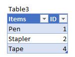
I'd like to be able to replace Count Pen, Count Stapler, Count Tape etc with 'cleverer' DAX that grabs the items of interest from a seperate table, like this:
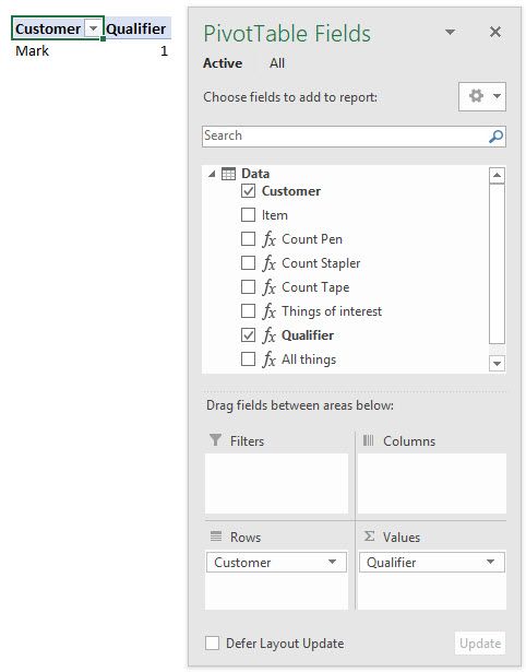
...and here's the result I'm after (using an Excel PivotTable):
Solved! Go to Solution.
- Mark as New
- Bookmark
- Subscribe
- Mute
- Subscribe to RSS Feed
- Permalink
- Report Inappropriate Content
You may refer to the following measure.
Measure =
VAR t =
    VALUES ( Table1[Item] )
RETURN
    IF (
        COUNTROWS ( Table1 ) = COUNTROWS ( t )
            && COUNTROWS ( Table1 ) = COUNTROWS ( Table2 )
            && ISEMPTY ( EXCEPT ( t, Table2 ) ),
        1
    )
If this post helps, then please consider Accept it as the solution to help the other members find it more quickly.
- Mark as New
- Bookmark
- Subscribe
- Mute
- Subscribe to RSS Feed
- Permalink
- Report Inappropriate Content
@v-chuncz-msft Works great in Excel 365. Unfortunately crashes my build of Excel 2016: I get a long delay when I try to commit the Measure, only to get a dialog saying:
Microsoft Excel is waiting for another application to complete an OLE Action
In the end I have to forcibly quit Excel. In fact, the only solution so far that I can get Excel 2016 to accept is the third one by @phil_seamark
Real pity that we get inconsistancies both across Excel/PBA as well as between Excel versions.
- Mark as New
- Bookmark
- Subscribe
- Mute
- Subscribe to RSS Feed
- Permalink
- Report Inappropriate Content
This is SOOO clever. I'm learning heaps from this, thanks. Hadn't come across the EXCEPT function before.
Phil Seamark has emailed me some approaches too, which I'll encourage him to post here. Turns out there are many ways to skin this particular cat.
- Mark as New
- Bookmark
- Subscribe
- Mute
- Subscribe to RSS Feed
- Permalink
- Report Inappropriate Content
Edit: Ignore this post. I had changed one of the columns from an int to text to simplify the example, but forgotton to refresh. Doh.
Hmmm...problem: Works great in PowerBI, doesn't work in Excel 365. I get an error " Function 'EXCEPT' does not support joining a column of type Text with a column of type Integer."
I've had the same from some of Phil Seamark's approaches too...despite the fact that all the approaches he's sent through work in PowerBI, some of his work only in Excel 365 but not Excel 2016, and some don't work in any version of Excel.
I'll write up Phil's approaches here when I get a chance, unless he beats me to it. It's an interesting formula challenge, and I'm sure others will be intrigued by the different approaches that can solve this, not to mention the different platforms that they do or don't work on.
- Mark as New
- Bookmark
- Subscribe
- Mute
- Subscribe to RSS Feed
- Permalink
- Report Inappropriate Content
Here's a few options that @Phil_Seamark was kind enough to email me when I spammed him. Looks like I'm buying him coffee tomorrow. Here's his first effort:
=
COUNTROWS (
    FILTER (
        SUMMARIZE (
            FILTER ( 'Table1', 'Table1'[Customer] = MAX ( 'Table1'[Customer] ) ),
            [Customer],
            "Total Items Purchased", DISTINCTCOUNT ( Table1[Item] ),
            "Distinct Preferred", COUNTROWS ( INTERSECT ( SELECTCOLUMNS ( Table1, "Items", [Item] ), Table2 ) )
        ),
        [Distinct Preferred] = [Total Items Purchased]
            && [Total Items Purchased] = COUNTROWS ( Table2 )
    )
)
Works great in PBI and Excel 365, but my build of Excel 2016 complains that The function MAX takes an argument that evaluates to numbers or dates and cannot work with values of type String.
Here's Phil's second offering:
=
VAR x =
    SELECTCOLUMNS (
        FILTER ( 'Table1', 'Table1'[Customer] = MAX ( 'Table1'[Customer] ) ),
        "Items", [Item]
    )
VAR y =
    UNION ( INTERSECT ( x, Items ), INTERSECT ( Items, x ) )
RETURN
    IF ( COUNTROWS ( y ) = COUNTROWS ( Items ) * 2, 1)
...which works great in PBI and Excel 365. But my build of Excel 2016 complains about MAX like the previous formula does.
His third one used the old parameter arg type trick of using 1, 2, 4, .... in a second column of Table2 so you could see if everything someone had purchased added to 7. Sneaky!
=COUNTROWS(
      FILTER(
        SUMMARIZE(
            'Table1',
            Table1[Customer],
            "Score", SUM('Table3'[ID]),
            "myRows",COUNTROWS('Table1')
       ),[Score]=SUM(Table3[ID]) && [myRows]=COUNTROWS(Table3))
     )
This works in both Excel 365 and my build of Excel 2016
Helpful resources

Microsoft Fabric Learn Together
Covering the world! 9:00-10:30 AM Sydney, 4:00-5:30 PM CET (Paris/Berlin), 7:00-8:30 PM Mexico City

Power BI Monthly Update - April 2024
Check out the April 2024 Power BI update to learn about new features.

| User | Count |
|---|---|
| 112 | |
| 97 | |
| 85 | |
| 67 | |
| 59 |
| User | Count |
|---|---|
| 150 | |
| 120 | |
| 100 | |
| 87 | |
| 68 |


