Excel Power Pivot. Related tables, pivot table repeats all row records

[Anonymous]

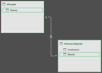
I have two tables that are connected by "Name." "People List" is a unique list of people, then "Responsibility" is accounts that they have ownership of:

Both tables are connected by "Name"

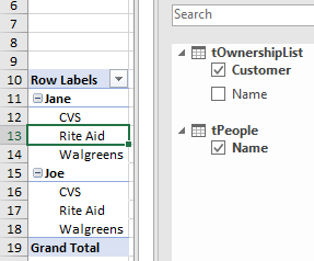
I need to organize it within a pivot table so that the "Name" comes from People table, and "Customer" from the Ownership list.

The problem that I'm experiencing is that when I drop these into the "rows" on my pivot table, account names repeat for each person.

How do I fix this so that only the assigned customers are visible for their respective people?

[itchyeyeballs]

What have you got in the values section of the pivot?

[Anonymous]

Currently, nothing.

[itchyeyeballs]

If you drop in name from your ownership table the extra rows should go away

[Anonymous]

Hm, it works, but in the true data I have a dozen measures that I drop in the data. It keeps repeating the customer name. I guess it's due to custom filters I have in some measures?

[itchyeyeballs]

Yes that can be an issue, are you using a function like all() in your measures? That can force results to be shown.

Can you share the Dax you are using in your measures?

[Anonymous]

Hm, found one that's causing this. When I divide two measures, then subtract 1 from the result, it starts showing every customer. Elaborate measure is below, but even if I reduce it to 

DIVIDE([ADS SALES], [(PY) ADS SALES], 0) - 1

it will create this behaviour of repeating customer names. If I only do the division, relationships work as expected.

=VAR ADS = DIVIDE([ADS SALES], [(PY) ADS SALES], 0)

RETURN
IF( OR( [(CY) SALES] <> 0, [(PY) SALES] <> 0 ),

  // corner case: if PY or CY is 0, then ADS will end up 0, but you want to capture growth,
  // which could be either -100%, or +100%
  IF( AND( [VARIANCE $ (SALES)] <> 0, ADS = 0), 
    [VARIANCE $ (SALES)] / ABS([VARIANCE $ (SALES)]),
    
    // not a corner case
    ADS - 1
  ),
  0
)

[itchyeyeballs]

Try replacing the 0 in divide function with blank() you don't need to specify 0 anyway as that's the default I think.

Edit - the minus 1 will likely produce a result for every possible combination and probably force a row to appear for each.

Blank - 1 = -1 (I think)

[Anonymous]

That seems to be the exact issue. Is there anything I can do to fix that? 

[itchyeyeballs · Accepted solution]

There's probably an elegant way to fix but my first thought is to add an isblank() check in an if statement.