- Power BI forums
- Updates
- News & Announcements
- Get Help with Power BI
- Desktop
- Service
- Report Server
- Power Query
- Mobile Apps
- Developer
- DAX Commands and Tips
- Custom Visuals Development Discussion
- Health and Life Sciences
- Power BI Spanish forums
- Translated Spanish Desktop
- Power Platform Integration - Better Together!
- Power Platform Integrations (Read-only)
- Power Platform and Dynamics 365 Integrations (Read-only)
- Training and Consulting
- Instructor Led Training
- Dashboard in a Day for Women, by Women
- Galleries
- Community Connections & How-To Videos
- COVID-19 Data Stories Gallery
- Themes Gallery
- Data Stories Gallery
- R Script Showcase
- Webinars and Video Gallery
- Quick Measures Gallery
- 2021 MSBizAppsSummit Gallery
- 2020 MSBizAppsSummit Gallery
- 2019 MSBizAppsSummit Gallery
- Events
- Ideas
- Custom Visuals Ideas
- Issues
- Issues
- Events
- Upcoming Events
- Community Blog
- Power BI Community Blog
- Custom Visuals Community Blog
- Community Support
- Community Accounts & Registration
- Using the Community
- Community Feedback
Register now to learn Fabric in free live sessions led by the best Microsoft experts. From Apr 16 to May 9, in English and Spanish.
- Power BI forums
- Forums
- Get Help with Power BI
- Desktop
- Re: Convert Excel Sumifs into DAX in Power bi
- Subscribe to RSS Feed
- Mark Topic as New
- Mark Topic as Read
- Float this Topic for Current User
- Bookmark
- Subscribe
- Printer Friendly Page
- Mark as New
- Bookmark
- Subscribe
- Mute
- Subscribe to RSS Feed
- Permalink
- Report Inappropriate Content
Convert Excel Sumifs into DAX in Power bi
Hi all
I am in the process of converting a data set in Excel to Power bi. I have done most of the transition but am stuck on this last part and its a huge value to me so I need to find a way to replicate.
Data set is attached:
I'll run through an example:
Row 4 in data set:
Company A have a line of revenue. They are paying £1000 for Product 1 to be delivered by P1 - Joe
Joe has therefore earnt £1000 from this line for Product 1
Row 5 in data set:
Company A has a 2nd line of revenue. This time worth £800 and it has been delivered by Ben and Joe
They therefore earn £400 each for Product 2
Joe has now earnt
£1000 - Product 1
£400 - Product 2
Ben has earnt
£400 - Product 2
I use excel to count and sumif the revenue by person by product, and then total in the table to the right of the data set.
How do i recreate this in Power bi?
Thanks
LOC
End result I'm after
- Mark as New
- Bookmark
- Subscribe
- Mute
- Subscribe to RSS Feed
- Permalink
- Report Inappropriate Content
Hi, @lea_313
Try to create a calculated table:
subTable =
var _t=ADDCOLUMNS(SELECTCOLUMNS('Table',"Product",[Product],"Revenue",[Revenue],"Number",[Numberofdeliversinvolved],"P1",[P1],"P2",[P2],"P3",[P3]),"Rev",DIVIDE([Revenue],[Number]))
var _t1=SELECTCOLUMNS(_t,"Product",[Product],"Name",[P1],"_Rev",[Rev])
var _t2=SELECTCOLUMNS(_t,"Product",[Product],"Name",[P2],"_Rev",[Rev])
var _t3=SELECTCOLUMNS(_t,"Product",[Product],"Name",[P3],"_Rev",[Rev])
var _tt=UNION(_t1,_t2,_t3)
return _tt
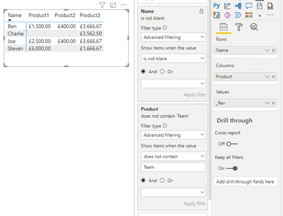
Then show data with a matrix.
Data:
Result:
Please refer to the attachment below for details. Hope this helps.
Best Regards,
Community Support Team _ Zeon Zheng
If this post helps, then please consider Accept it as the solution to help the other members find it more quickly.
- Mark as New
- Bookmark
- Subscribe
- Mute
- Subscribe to RSS Feed
- Permalink
- Report Inappropriate Content
Hiya
Thanks for this, this has worked but I am stuck at 1 issue.
My 'people' have 2 ID numbers, so when I use your calculation above I then get incorrect results.
I need to add a column that converts the ID numbers to a single name as shown in the column below 'calculation I need'
Could you help with this please?
thanks so much
- Mark as New
- Bookmark
- Subscribe
- Mute
- Subscribe to RSS Feed
- Permalink
- Report Inappropriate Content
Thanks for the reply
How do I calculate the number of deliverers involved? I currently need to count columns per row where 3 columns of potential deliverers is not empty. My deliverers show as an ID number too which makes it complicated.
Deliverer 1 - 45
Deliverer 2 - 42
Deliverer 1 - 31
These are all seperate columns, I need something to count 3 columns have entires so there are 3 deliverers involved here
thanks
lea
- Mark as New
- Bookmark
- Subscribe
- Mute
- Subscribe to RSS Feed
- Permalink
- Report Inappropriate Content
@lea_313 can you provide sample data rpresentative of your issue here that can be easily copy pasted in Power BI (in table format) and also clearly show your desired output.
- Mark as New
- Bookmark
- Subscribe
- Mute
- Subscribe to RSS Feed
- Permalink
- Report Inappropriate Content
Hiya
Details below
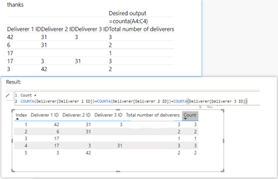
Desired output shown in column 4 and the formula I use in excel
thanks
| Desired output | |||
| =counta(A4:C4) | |||
| Deliverer 1 ID | Deliverer 2 ID | Deliverer 3 ID | Total number of deliverers |
| 42 | 31 | 3 | 3 |
| 6 | 31 | 2 | |
| 17 | 1 | ||
| 17 | 3 | 31 | 3 |
| 3 | 42 | 2 |
- Mark as New
- Bookmark
- Subscribe
- Mute
- Subscribe to RSS Feed
- Permalink
- Report Inappropriate Content
Hi, @lea_313
Is the above formula useful to you? My efforts are meaningful if it is helpful to you and you will be consider marking it as Answered since it is working now.
Regarding your current question, if I understand your question correctly, please use the following formula.
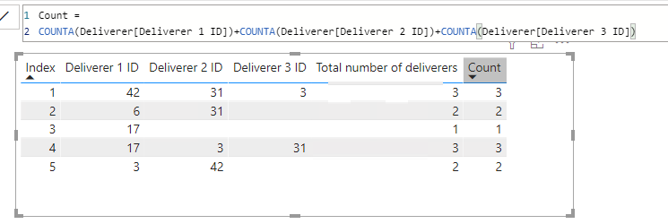
Count =
COUNTA(Deliverer[Deliverer 1 ID])+COUNTA(Deliverer[Deliverer 2 ID])+COUNTA(Deliverer[Deliverer 3 ID])
Result:
Best Regards,
Community Support Team _ Zeon Zheng
If this post helps, then please consider Accept it as the solution to help the other members find it more quickly.
- Mark as New
- Bookmark
- Subscribe
- Mute
- Subscribe to RSS Feed
- Permalink
- Report Inappropriate Content
Hiya
This doesnt seem to do the calculation per row? I just get a total for the whole column?
Thanks
- Mark as New
- Bookmark
- Subscribe
- Mute
- Subscribe to RSS Feed
- Permalink
- Report Inappropriate Content
Hi, @lea_313
This makes me a little confused, is this not what you want?
If not, could you please consdier sharing more details about it and posting expected result so it is clear on what needs to be implemented?
If I can be absolutely clear about what you want to do, I think I might get a solution.
And it would be great if my first formula can work for your initial problem.
Best Regards,
Community Support Team _ Zeon Zheng
If this post helps, then please consider Accept it as the solution to help the other members find it more quickly.
- Mark as New
- Bookmark
- Subscribe
- Mute
- Subscribe to RSS Feed
- Permalink
- Report Inappropriate Content
I would like to make a column that based on the id I calculate the days of the month that that person attended.
- Mark as New
- Bookmark
- Subscribe
- Mute
- Subscribe to RSS Feed
- Permalink
- Report Inappropriate Content
Hi @lea_313 ,
Try the following in Power Query:
1. Divide the amount with the number of people:
2. Select P1, P2 & P3, then press unpivot columns in the transform tab:
3. Remove empty rows in the value column:
4. Remove or rename the old Amount column, rename the division column:
Hope this helps,
/ J
- Mark as New
- Bookmark
- Subscribe
- Mute
- Subscribe to RSS Feed
- Permalink
- Report Inappropriate Content
Hiya
Just wanted to say I really appreciated your detailed reply! The pictures made it a lot easier to follow thank you
I ended up having issues at the unpivot section. This seemed to not be possible the data I had so I have used the above formula to create a subtable.
I have hit another small hurdle,
My 'people' have 2 ID numbers, so when I use a calculation above I then get incorrect results.
I need to add a column that converts the ID numbers to a single name as shown in the column below 'calculation I need'
Could you help with this please?
thanks so much
Thanks
Lea
- Mark as New
- Bookmark
- Subscribe
- Mute
- Subscribe to RSS Feed
- Permalink
- Report Inappropriate Content
Hi
Wow thank you for such a detailed response!!
Looks great, I just got a bit stuck at the first hurdle sorry
I dont have number of people as a column in my data. I should have explained anything past the yellow column is a calculation in my spreadsheet.
Also, to complicate things, people in my data show up as an ID number.
So for Row 2, i dont want to sum the rows (i.e. 4+13), i just need it to say 2 non blank cells = 2 people involved
Hope this is clear
thanks, really appreciate your help
Lea
- Mark as New
- Bookmark
- Subscribe
- Mute
- Subscribe to RSS Feed
- Permalink
- Report Inappropriate Content
Hi Lea,
You should be able to use the following column i power Query to make your own "Number of people" column:
let
p1 = if [P1] = null then 0 else 1,
p2 = if [P2] = null then 0 else 1,
p3 = if [P3] = null then 0 else 1
in
p1+p2+p3
Br,
J
Connect on LinkedIn
- Mark as New
- Bookmark
- Subscribe
- Mute
- Subscribe to RSS Feed
- Permalink
- Report Inappropriate Content
Hiya
Thanks again for your reply
I just get an error that I have mistyped the column name but I'm using them from the Available columns table on the right of the image you sent above. That or an error saying Token Eof Expected
Image below, I've copied your formula to my actual data but it's not going through. Really do appreicate the help thanks
Thanks so much
- Mark as New
- Bookmark
- Subscribe
- Mute
- Subscribe to RSS Feed
- Permalink
- Report Inappropriate Content
Hi Lea,
The code needs to be precise, the reason it's not working is because you're using a capital "L" in the beginning, giving you "Let" instead of "let".
Your code should look like this i believe:
let
DelivererId = if [DelivererId] = null then 0 else 1,
CoDelivererId = if [CoDelivererId] = null then 0 else 1,
CoDeliverer2Id = if [CoDeliverer2Id] = null then 0 else 1
in
DelivererId+CoDelivererId+CoDeliverer2Id
Br,
J
Connect on LinkedIn
- Mark as New
- Bookmark
- Subscribe
- Mute
- Subscribe to RSS Feed
- Permalink
- Report Inappropriate Content
Hi @lea_313 ,
Try the following in Power Query:
1. Divide the amount with the number of people:
2. Select P1, P2 & P3, then press unpivot columns in the transform tab:
3. Remove empty rows in the value column:
4. Remove or rename the old Amount column, rename the division column:
Hope this helps,
/ J
Connect on LinkedIn
Helpful resources

Microsoft Fabric Learn Together
Covering the world! 9:00-10:30 AM Sydney, 4:00-5:30 PM CET (Paris/Berlin), 7:00-8:30 PM Mexico City

Power BI Monthly Update - April 2024
Check out the April 2024 Power BI update to learn about new features.

| User | Count |
|---|---|
| 110 | |
| 96 | |
| 77 | |
| 63 | |
| 55 |
| User | Count |
|---|---|
| 143 | |
| 109 | |
| 89 | |
| 84 | |
| 66 |


