- Power BI forums
- Updates
- News & Announcements
- Get Help with Power BI
- Desktop
- Service
- Report Server
- Power Query
- Mobile Apps
- Developer
- DAX Commands and Tips
- Custom Visuals Development Discussion
- Health and Life Sciences
- Power BI Spanish forums
- Translated Spanish Desktop
- Power Platform Integration - Better Together!
- Power Platform Integrations (Read-only)
- Power Platform and Dynamics 365 Integrations (Read-only)
- Training and Consulting
- Instructor Led Training
- Dashboard in a Day for Women, by Women
- Galleries
- Community Connections & How-To Videos
- COVID-19 Data Stories Gallery
- Themes Gallery
- Data Stories Gallery
- R Script Showcase
- Webinars and Video Gallery
- Quick Measures Gallery
- 2021 MSBizAppsSummit Gallery
- 2020 MSBizAppsSummit Gallery
- 2019 MSBizAppsSummit Gallery
- Events
- Ideas
- Custom Visuals Ideas
- Issues
- Issues
- Events
- Upcoming Events
- Community Blog
- Power BI Community Blog
- Custom Visuals Community Blog
- Community Support
- Community Accounts & Registration
- Using the Community
- Community Feedback
Register now to learn Fabric in free live sessions led by the best Microsoft experts. From Apr 16 to May 9, in English and Spanish.
- Power BI forums
- Forums
- Get Help with Power BI
- Desktop
- POWERBI NEWBIE HELP
- Subscribe to RSS Feed
- Mark Topic as New
- Mark Topic as Read
- Float this Topic for Current User
- Bookmark
- Subscribe
- Printer Friendly Page
- Mark as New
- Bookmark
- Subscribe
- Mute
- Subscribe to RSS Feed
- Permalink
- Report Inappropriate Content
POWERBI NEWBIE HELP
Hello,
I'm really new in using PowerBI and I'm just trying to study functions and create reports of future implementation.
Some background:
The data I have is already around 500,000 rows. My month column is formatted as YYYY/MM and read as MM/DD/YYYY by PowerBI. All the DDs are 1 since there are no dates. Weeks are formatted as YYYY/WW, but read as WW/DD/YYYY.
I tried using delimeter to create a separate week and month column through query. If I'm not mistaken, I read that I have to duplicate of my current master query and manipulate from there. After creating the three new columns, I removed other columns for easier loading. I don't know if this is right.
After trying to apply, I get this error on the values of my Week column although its format is already a whole number
"DataFormat.Error: We couldn't parse the input provided as a Date value.
Details:
2015/13"
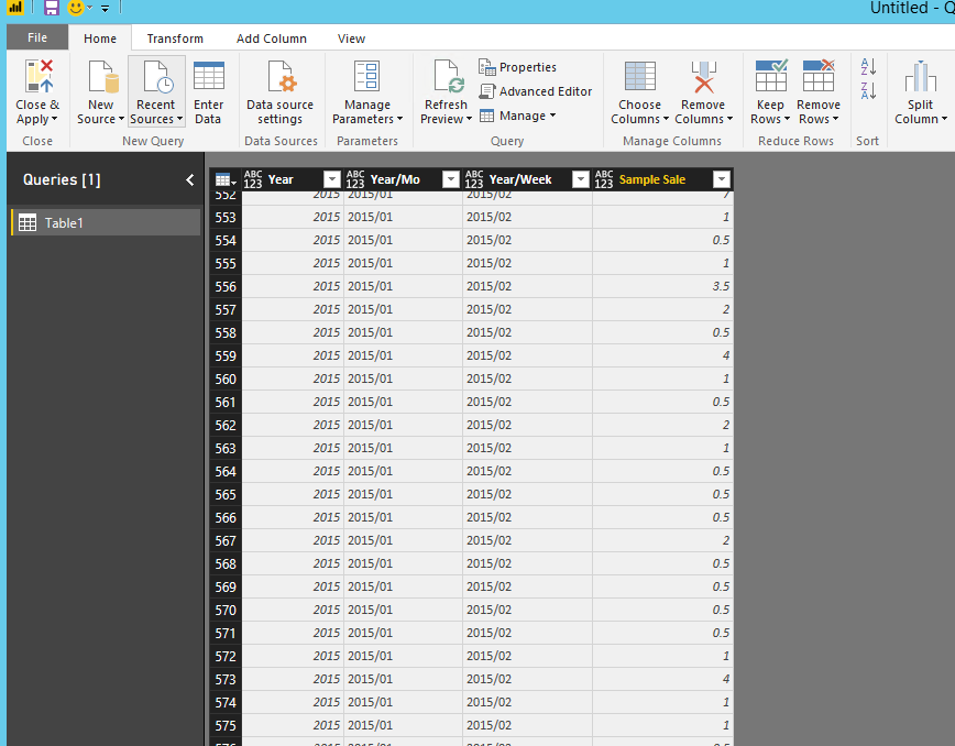
Also, another thing: PowerBI adds a row number column automatically with weird numbers. Is that normal? Do I delete it? Is it related to the indexing, something I read online as well? Thank you guys so much in advance.
----
Hope you guys can help. I have so much questions and I hope this website can guide me through.
Solved! Go to Solution.
- Mark as New
- Bookmark
- Subscribe
- Mute
- Subscribe to RSS Feed
- Permalink
- Report Inappropriate Content
@jansenuy wrote:
Hello @Eric_Zhang
I am sending the excel file. Hope you can import it to a new pbix file because mine currently is very messy already as I tried experimenting on things. I'm really new at this so sorry about that. Again my three main issues are:
1. The row numbers added upon importation of the excel.
2. How to have separate week, year, and month columns?
3. Although I was able to delimit the week column into just plain numbers of 1,2,3,...53, it presents the parsing error upon applying the query.
4. Properly create charts that would present sales weekly in 2017 and 2016
https://www.sendspace.com/file/3ms5c2
Thank you again
Thanks for sharing the file! 🙂
Based on my test, to import the excel in a good way, you can follow below steps.
- Open Power BI desktop.
- Go to "File"->"Options and settings"->"Options"-> "Current File"->"Data Load" and uncheck "Automatically detect column types and header for unstructed sources" and "Auto Date/Time". Then click "OK".
- "Get data"->excel and load your file, check "Table1" and click "Editor" to go to Query Editor.
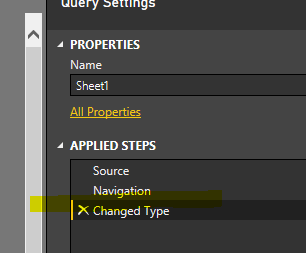
- Remove the step "Changed Type". Then you get the data imported correctly without any messy row number column.
To split Year/Week, click "Split column"
Change the sample sale to decimal type.
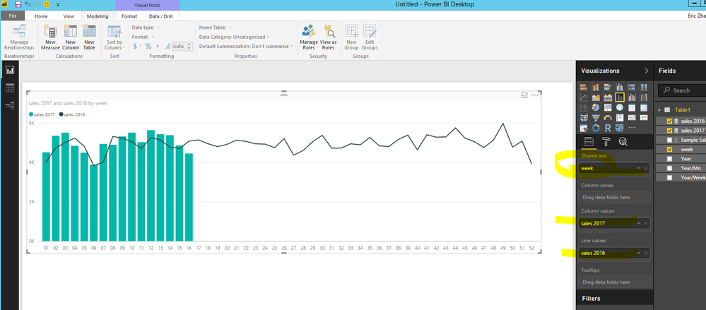
I'm trying to create a graph with 2016 sales values and 2017 sales values weekly. The 2016 values from weeks 1 to 52 are in line bar while the 2017 values are progressing above in a line.
Then create two measures
sales 2016 = CALCULATE(sum(Table1[Sample Sale]),FILTER(Table1,Table1[Year]="2016"))

sales 2017 = CALCULATE(sum(Table1[Sample Sale]),FILTER(Table1,Table1[Year]="2017"))
Attached PBIX file for your reference.
- Mark as New
- Bookmark
- Subscribe
- Mute
- Subscribe to RSS Feed
- Permalink
- Report Inappropriate Content
@jansenuy wrote:
Hello,
I'm really new in using PowerBI and I'm just trying to study functions and create reports of future implementation.
Some background:
The data I have is already around 500,000 rows. My month column is formatted as YYYY/MM and read as MM/DD/YYYY by PowerBI. All the DDs are 1 since there are no dates. Weeks are formatted as YYYY/WW, but read as WW/DD/YYYY.
I tried using delimeter to create a separate week and month column through query. If I'm not mistaken, I read that I have to duplicate of my current master query and manipulate from there. After creating the three new columns, I removed other columns for easier loading. I don't know if this is right.
After trying to apply, I get this error on the values of my Week column although its format is already a whole number
"DataFormat.Error: We couldn't parse the input provided as a Date value.
Details:
2015/13"
Also, another thing: PowerBI adds a row number column automatically with weird numbers. Is that normal? Do I delete it? Is it related to the indexing, something I read online as well? Thank you guys so much in advance.
----
Hope you guys can help. I have so much questions and I hope this website can guide me through.
To avoid the auto conversion, you could go to "File"->"Options"->"Data Load" and uncheck the "Type detection".
For weird numbers, could you post a snapshot to show more details?
- Mark as New
- Bookmark
- Subscribe
- Mute
- Subscribe to RSS Feed
- Permalink
- Report Inappropriate Content
For the weird numbers, it's just a generated column titled Row Number then with random counting numbers as values. It's like it's trying to put a row number. It first happens when I imported Excel data into PowerBI. But instead of starting with 1 as row number, it starts with like 850 or 7493 some random start. I just delete it because I feel like it doesn't make sense since there is a row number in query mode anyway.
Regarding your solution, it did solve my error. Any reason behind that so I know in the future?
Also,
I'm trying to create a graph with 2016 sales values and 2017 sales values weekly. The 2016 values from weeks 1 to 52 are in line bar while the 2017 values are progressing above in a line. My data is like this:
Year Month Week Sales
2016 1 1 xxxx
...
2016 2 5 xxxx
...
2017 12 53 xxxx
Hope you get the idea above. I'm having a hard time choosing the right fields to put in the line and clustered column chart. Totally a noob. 😞 Thanks in advance.
- Mark as New
- Bookmark
- Subscribe
- Mute
- Subscribe to RSS Feed
- Permalink
- Report Inappropriate Content
@jansenuy wrote:
For the weird numbers, it's just a generated column titled Row Number then with random counting numbers as values. It's like it's trying to put a row number. It first happens when I imported Excel data into PowerBI. But instead of starting with 1 as row number, it starts with like 850 or 7493 some random start. I just delete it because I feel like it doesn't make sense since there is a row number in query mode anyway.
Regarding your solution, it did solve my error. Any reason behind that so I know in the future?
Also,
I'm trying to create a graph with 2016 sales values and 2017 sales values weekly. The 2016 values from weeks 1 to 52 are in line bar while the 2017 values are progressing above in a line. My data is like this:
Year Month Week Sales
2016 1 1 xxxx
...
2016 2 5 xxxx
...
2017 12 53 xxxx
Hope you get the idea above. I'm having a hard time choosing the right fields to put in the line and clustered column chart. Totally a noob. 😞 Thanks in advance.
With that option checked, Power BI desktop will try to understand and convert the data into proper types. You can also revert the conversion by deleting the changed types step.
I'm not yet able to get the weird numbers in my test, maybe you can share me your pbix file?
As to 2016 and 2017 question, you can try to put the Week as X-AXIS and create two measure with filters like below and put them to line values and column values accordingly.
2017 measure = calculate(SUM(table[Sales]),FILER('table',Max(table[Year])=2017))


2016 measure = calculate(SUM(table[Sales]),FILER('table',Max(table[Year])=2016))
- Mark as New
- Bookmark
- Subscribe
- Mute
- Subscribe to RSS Feed
- Permalink
- Report Inappropriate Content
Hi @Eric_Zhang thanks for your patience. Please see link to the download the error pictures. Apparently, the first error wasn't solved. Picture 1 shows that. Picture 2 shows the error with your code. Thanks.
- Mark as New
- Bookmark
- Subscribe
- Mute
- Subscribe to RSS Feed
- Permalink
- Report Inappropriate Content
- Mark as New
- Bookmark
- Subscribe
- Mute
- Subscribe to RSS Feed
- Permalink
- Report Inappropriate Content
@jansenuy wrote:
@Eric_Zhang Sorry here it is https://www.sendspace.com/filegroup/emrU%2FMROfd1E%2FD6g5dTPTQ
The snapshot doesn't help too much, is it possible to share the pbix file and your excel?
- Mark as New
- Bookmark
- Subscribe
- Mute
- Subscribe to RSS Feed
- Permalink
- Report Inappropriate Content
Hello @Eric_Zhang
I am sending the excel file. Hope you can import it to a new pbix file because mine currently is very messy already as I tried experimenting on things. I'm really new at this so sorry about that. Again my three main issues are:
1. The row numbers added upon importation of the excel.
2. How to have separate week, year, and month columns?
3. Although I was able to delimit the week column into just plain numbers of 1,2,3,...53, it presents the parsing error upon applying the query.
4. Properly create charts that would present sales weekly in 2017 and 2016
https://www.sendspace.com/file/3ms5c2
Thank you again
- Mark as New
- Bookmark
- Subscribe
- Mute
- Subscribe to RSS Feed
- Permalink
- Report Inappropriate Content
@jansenuy wrote:
Hello @Eric_Zhang
I am sending the excel file. Hope you can import it to a new pbix file because mine currently is very messy already as I tried experimenting on things. I'm really new at this so sorry about that. Again my three main issues are:
1. The row numbers added upon importation of the excel.
2. How to have separate week, year, and month columns?
3. Although I was able to delimit the week column into just plain numbers of 1,2,3,...53, it presents the parsing error upon applying the query.
4. Properly create charts that would present sales weekly in 2017 and 2016
https://www.sendspace.com/file/3ms5c2
Thank you again
Thanks for sharing the file! 🙂
Based on my test, to import the excel in a good way, you can follow below steps.
- Open Power BI desktop.
- Go to "File"->"Options and settings"->"Options"-> "Current File"->"Data Load" and uncheck "Automatically detect column types and header for unstructed sources" and "Auto Date/Time". Then click "OK".
- "Get data"->excel and load your file, check "Table1" and click "Editor" to go to Query Editor.
- Remove the step "Changed Type". Then you get the data imported correctly without any messy row number column.
To split Year/Week, click "Split column"
Change the sample sale to decimal type.
I'm trying to create a graph with 2016 sales values and 2017 sales values weekly. The 2016 values from weeks 1 to 52 are in line bar while the 2017 values are progressing above in a line.
Then create two measures
sales 2016 = CALCULATE(sum(Table1[Sample Sale]),FILTER(Table1,Table1[Year]="2016"))

sales 2017 = CALCULATE(sum(Table1[Sample Sale]),FILTER(Table1,Table1[Year]="2017"))
Attached PBIX file for your reference.
- Mark as New
- Bookmark
- Subscribe
- Mute
- Subscribe to RSS Feed
- Permalink
- Report Inappropriate Content
Thank you so much!!!!!!! I was able to generate the graph. What if I would be filtering two items from one column? How would I combine them? I tried using parenthesis, adding the word "and" and using && 😞 @Eric_Zhang
- Mark as New
- Bookmark
- Subscribe
- Mute
- Subscribe to RSS Feed
- Permalink
- Report Inappropriate Content
@jansenuy wrote:
Thank you so much!!!!!!! I was able to generate the graph. What if I would be filtering two items from one column? How would I combine them? I tried using parenthesis, adding the word "and" and using && 😞 @Eric_Zhang
what column would you like to use to filter those two measures?
- Mark as New
- Bookmark
- Subscribe
- Mute
- Subscribe to RSS Feed
- Permalink
- Report Inappropriate Content
@Eric_Zhang I just have a bigger dataset with a location column and I need to filter 2 or more locations
- Mark as New
- Bookmark
- Subscribe
- Mute
- Subscribe to RSS Feed
- Permalink
- Report Inappropriate Content
@jansenuy wrote:
@Eric_Zhang I just have a bigger dataset with a location column and I need to filter 2 or more locations
Then I think those two measure shall work. Have you got any issue?
- Mark as New
- Bookmark
- Subscribe
- Mute
- Subscribe to RSS Feed
- Permalink
- Report Inappropriate Content
@Eric_Zhang Ended up with this and it got kinda confusing resulting to an error that said too few arguments passed to the filter function:
Don't know if I applied correctly. Thanks
- Mark as New
- Bookmark
- Subscribe
- Mute
- Subscribe to RSS Feed
- Permalink
- Report Inappropriate Content
@jansenuy wrote:
@Eric_Zhang Ended up with this and it got kinda confusing resulting to an error that said too few arguments passed to the filter function:
SpoilerSalesA2016 = CALCULATE(SUM('Master Data'[Sales]),FILTER('Master Data','Master Data'[Year]="2016"), FILTER('Master Data'[Destination]in {"US","UK"}),FILTER('Master Data'[Selling Country]="Philippines"))Don't know if I applied correctly. Thanks
It is some syntax error, try
SalesA2016 =
CALCULATE (
    SUM ( 'Master Data'[Sales] ),
    FILTER ( 'Master Data', 'Master Data'[Year] = "2016" ),
    FILTER ( 'Master Data', 'Master Data'[Destination] IN { "US", "UK" } ),
    FILTER ( 'Master Data', 'Master Data'[Selling Country] = "Philippines" )
)
By the way, you can apply the destination and country in slicers instead of hard coded them in the measures.
Also a good DAX Formatter site FYI.
- Mark as New
- Bookmark
- Subscribe
- Mute
- Subscribe to RSS Feed
- Permalink
- Report Inappropriate Content
sales 2017 /2017= CALCULATE(sum(Table1[Sample Sale]),Table1[Year]in {"2017","2016"})
or
sales 2017 /2017= CALCULATE(sum(Table1[Sample Sale]),Table1[Year] = "2017" ||
Table1[Year] = "2016")
If I took the time to answer your question and I came up with a solution, please mark my post as a solution and /or give kudos freely for the effort 🙂 Thank you!
Proud to be a Super User!
- Mark as New
- Bookmark
- Subscribe
- Mute
- Subscribe to RSS Feed
- Permalink
- Report Inappropriate Content
Helpful resources

Microsoft Fabric Learn Together
Covering the world! 9:00-10:30 AM Sydney, 4:00-5:30 PM CET (Paris/Berlin), 7:00-8:30 PM Mexico City

Power BI Monthly Update - April 2024
Check out the April 2024 Power BI update to learn about new features.

| User | Count |
|---|---|
| 109 | |
| 98 | |
| 80 | |
| 64 | |
| 57 |
| User | Count |
|---|---|
| 145 | |
| 110 | |
| 91 | |
| 84 | |
| 66 |


